Space 概念详解

Space 概念：完整的 3D 图像几何描述

每一幅医学图像都对应物理世界中的一个规范采样网格。SpaceTransformer 通过 Space 对象的六个要素来完整描述这个网格：形状、原点、间距与三个方向向量。

import numpy as np
import matplotlib.pyplot as plt
from spacetransformer.core import Space

# 创建一个标准的规范采样网格
standard_space = Space(
    shape=(1, 10, 10),               # 三维网格，第一维度为1用于2D可视化
    origin=(0.0, 0.0, 0.0),          # 物理原点
    spacing=(1.0, 1.0, 1.0),         # 各向同性1mm采样
    x_orientation=(1.0, 0.0, 0.0),   # X轴方向
    y_orientation=(0.0, 1.0, 0.0),   # Y轴方向  
    z_orientation=(0.0, 0.0, 1.0)    # Z轴方向
)

# 展示标准规范采样网格

为了直观展示 Space 变换效果，我们实现 2D 网格可视化：

def visualize_sampling_grid(space, color='blue', show_axes=True, label_suffix=''):
    """
    可视化采样网格的2D投影（绘制所有采样点）
    
    Args:
        space: Space 对象
        color: 绘制颜色
        show_axes: 是否显示坐标轴
        label_suffix: 标签后缀，用于区分不同的网格
    """
    # 提取 Y-Z 平面信息（忽略 X 维）
    shape_yz = space.shape[1:3]  # (height, width)
    
    # 创建所有索引点的网格
    y_indices, z_indices = np.meshgrid(
        np.arange(shape_yz[0]),
        np.arange(shape_yz[1]),
        indexing='ij'
    )
    
    # 构建 3D 索引点（X 维设为 0）
    index_points = np.stack([
        np.zeros_like(y_indices.flatten()),  # X=0
        y_indices.flatten(),                 # Y索引
        z_indices.flatten()                  # Z索引
    ], axis=1)
    
    # 转换为世界坐标
    world_points = space.to_world_transform.apply_point(index_points)
    
    # 绘制采样点
    plt.scatter(world_points[:, 2], world_points[:, 1], 
               c=color, alpha=0.4, s=20, label=f'Sampling Grid{label_suffix}')
    
    if show_axes:
        # 显示原点和坐标轴方向
        origin_world = space.to_world_transform.apply_point([[0, 0, 0]])[0]
        plt.plot(origin_world[2], origin_world[1], 'o', 
                color=color, markersize=8, alpha=0.8)
        
        # 计算坐标轴长度（适当拉长）
        axis_length = 1
        
        # Y 轴方向（图中为垂直）
        y_axis_end = origin_world[1:3] + np.array(space.y_orientation[1:3]) * axis_length
        plt.arrow(origin_world[2], origin_world[1], 
                 y_axis_end[1] - origin_world[2], y_axis_end[0] - origin_world[1],
                 head_width=axis_length*0.1, head_length=axis_length*0.1, 
                 fc=color, ec=color, alpha=0.7)
        
        # Y轴文字标注（偏移避免被箭头遮挡）
        y_text_offset = np.array(space.y_orientation[1:3]) * axis_length * 0.3
        plt.text(y_axis_end[1] + y_text_offset[1], y_axis_end[0] + y_text_offset[0], 'Y', 
                fontsize=12, color=color, ha='center', va='center', weight='bold')
        
        # Z 轴方向（图中为水平）
        z_axis_end = origin_world[1:3] + np.array(space.z_orientation[1:3]) * axis_length
        plt.arrow(origin_world[2], origin_world[1],
                 z_axis_end[1] - origin_world[2], z_axis_end[0] - origin_world[1],
                 head_width=axis_length*0.1, head_length=axis_length*0.1,
                 fc=color, ec=color, alpha=0.7)
        
        # Z轴文字标注（偏移避免被箭头遮挡）
        z_text_offset = np.array(space.z_orientation[1:3]) * axis_length * 0.3
        plt.text(z_axis_end[1] + z_text_offset[1], z_axis_end[0] + z_text_offset[0], 'Z', 
                fontsize=12, color=color, ha='center', va='center', weight='bold')

def setup_plot(figsize=(10, 8)):
    """设置绘图通用参数"""
    plt.figure(figsize=figsize)

def finalize_plot(title):
    """完成绘图的通用设置"""
    plt.xlabel('Z (mm)')
    plt.ylabel('Y (mm)')
    plt.title(title)
    plt.grid(True, alpha=0.3)
    plt.axis('equal')
    plt.legend()
    plt.tight_layout()
    plt.show()

# 可视化标准网格
setup_plot()
visualize_sampling_grid(standard_space, color='blue')
finalize_plot('Standard Sampling Grid (10x10, 1mm resolution)')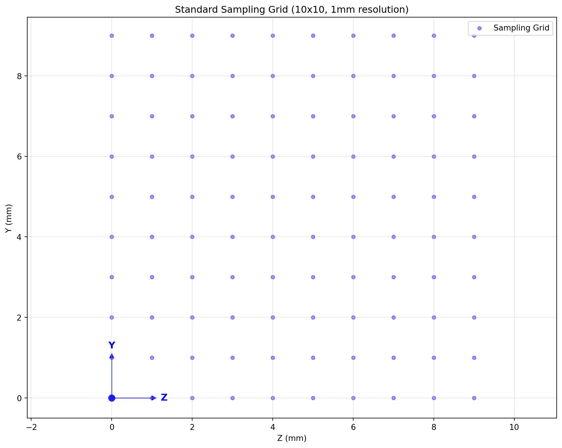

空间变换操作演示

形状变换（Resize）

# 创建不同分辨率的采样网格
high_res_space = standard_space.apply_shape((1, 20, 20))
low_res_space = standard_space.apply_shape((1, 5, 5))

setup_plot()
# 低分辨率对比
visualize_sampling_grid(standard_space, color='blue', label_suffix=' (Original)')
visualize_sampling_grid(low_res_space, color='red', label_suffix=' (5x5)')
finalize_plot('Low Resolution Transform (10x10 → 5x5)')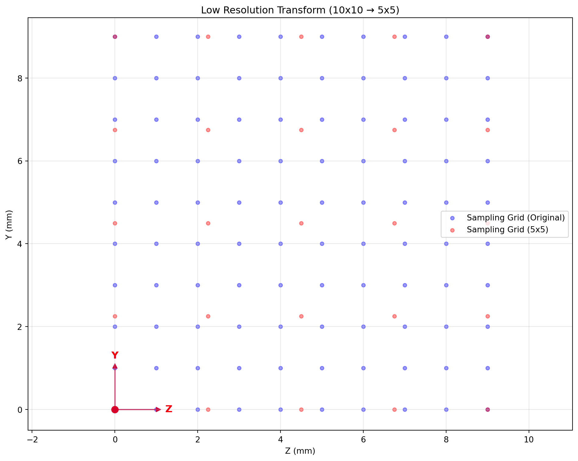

翻转变换

# 创建翻转的采样网格
flipped_space = standard_space.apply_flip(axis=1)  # 沿Y轴翻转

# 可视化翻转变换的overlay效果
setup_plot()
visualize_sampling_grid(standard_space, color='blue', label_suffix=' (Original)')
visualize_sampling_grid(flipped_space, color='red', label_suffix=' (Flipped Y-axis)')
finalize_plot('Flip Transform (Y-axis)')

轴交换变换

# 创建轴交换的采样网格（使用非正方形网格以增强对比）
rect_space = Space(
    shape=(1, 6, 12),  # 矩形网格
    origin=(0.0, 0.0, 0.0),
    spacing=(1.0, 1.0, 1.0),
    x_orientation=(1.0, 0.0, 0.0),
    y_orientation=(0.0, 1.0, 0.0),
    z_orientation=(0.0, 0.0, 1.0)
)

swapped_space = rect_space.apply_swap(1, 2)  # 交换 Y 轴与 Z 轴

# 可视化轴交换变换的overlay效果
setup_plot()
visualize_sampling_grid(rect_space, color='blue', label_suffix=' (Original 6x12)')
visualize_sampling_grid(swapped_space, color='red', label_suffix=' (Swapped Y↔Z 12x6)')
finalize_plot('Axis Swap Transform (Y ↔ Z)')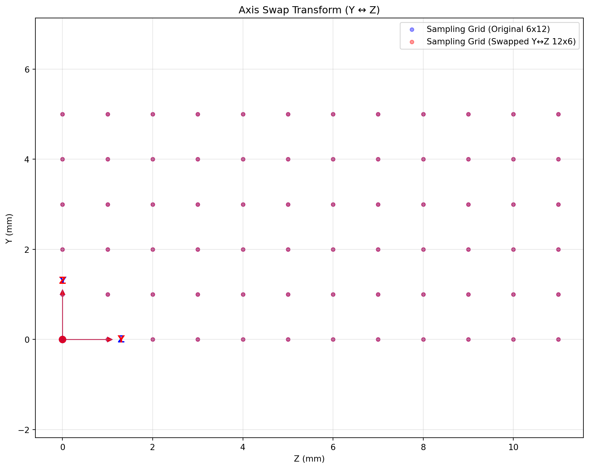

旋转变换

# 创建旋转的采样网格
rotated_space = standard_space.apply_rotate(axis=0, angle=30, unit='degree', center='center')

# 可视化旋转变换的overlay效果
setup_plot()
visualize_sampling_grid(standard_space, color='blue', label_suffix=' (Original)')
visualize_sampling_grid(rotated_space, color='red', label_suffix=' (Rotated 30°)')
finalize_plot('Rotation Transform (around X-axis 30°)')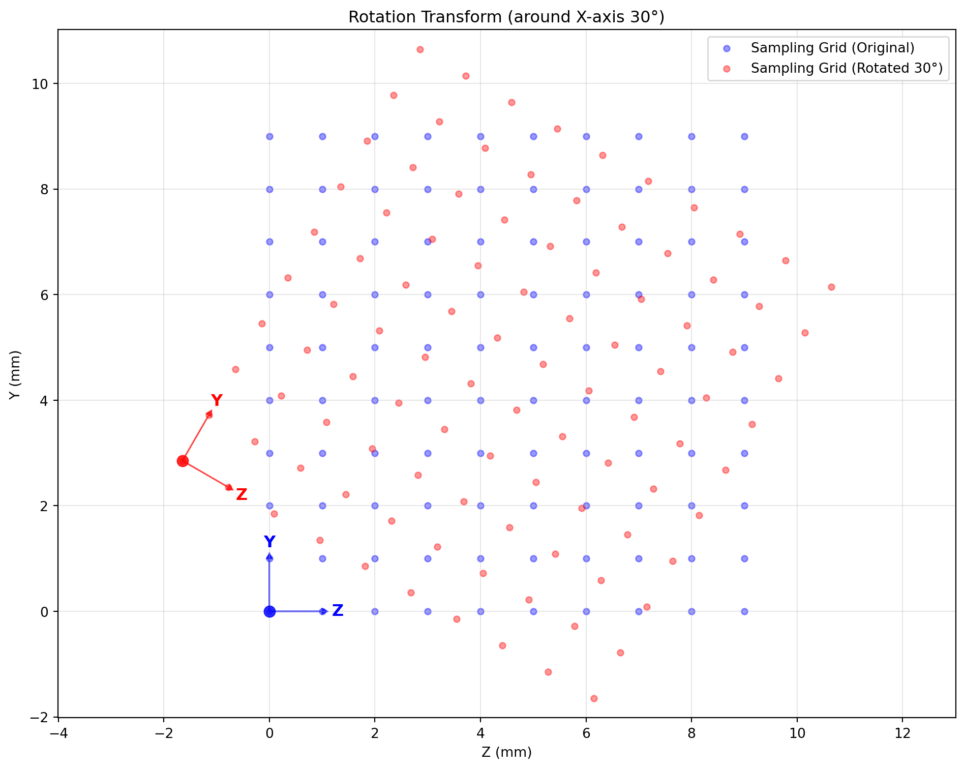

边界框裁剪

# 定义裁剪区域并应用变换
crop_bbox = np.array([[0, 1], [2, 8], [2, 8]])  # X, Y, Z范围
cropped_space = standard_space.apply_bbox(crop_bbox)

# 可视化裁剪变换的overlay效果
setup_plot()
visualize_sampling_grid(standard_space, color='blue', label_suffix=' (Original)')
visualize_sampling_grid(cropped_space, color='red', label_suffix=' (Cropped ROI)')
finalize_plot('Bounding Box Crop (6x6 ROI)')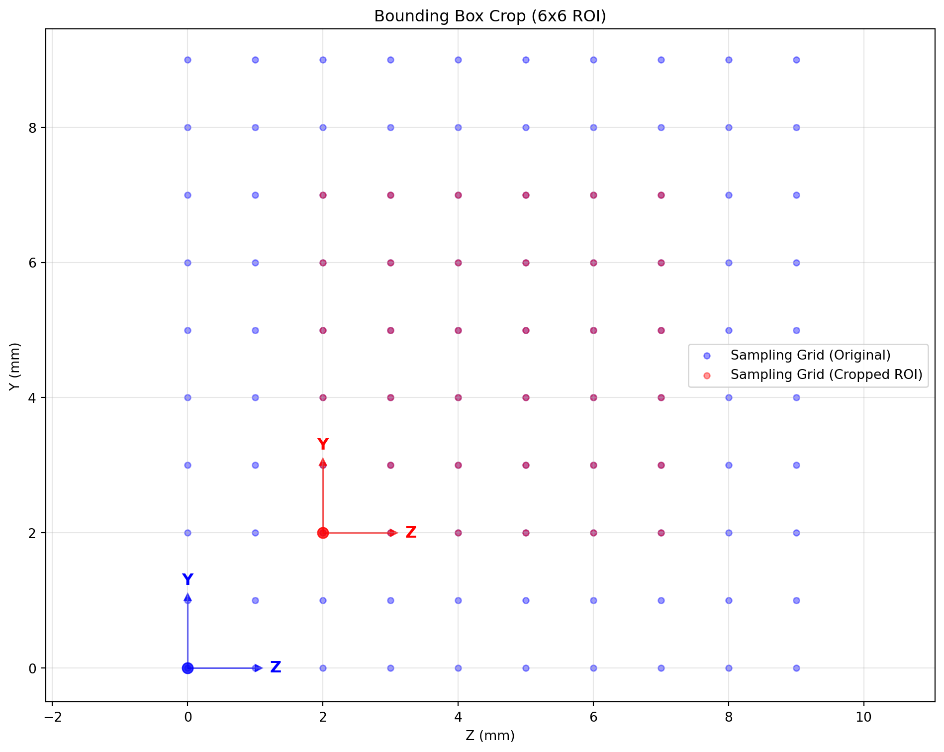

复杂变换链

# 演示复杂变换链的抽象规划
complex_target_space = (standard_space
    .apply_bbox(np.array([[0, 1], [2, 8], [2, 8]]))  # 裁剪到中心区域
    .apply_shape((1, 12, 12))                         # 重采样到12×12
    .apply_rotate(axis=0, angle=45, unit='degree')    # 旋转45度
)

# 可视化复杂变换链的 overlay 效果
setup_plot()
visualize_sampling_grid(standard_space, color='blue', label_suffix=' (Original)')
visualize_sampling_grid(complex_target_space, color='red', label_suffix=' (Crop→Resample→Rotate)')
finalize_plot('Complex Transform Chain (Crop → Resample → Rotate)')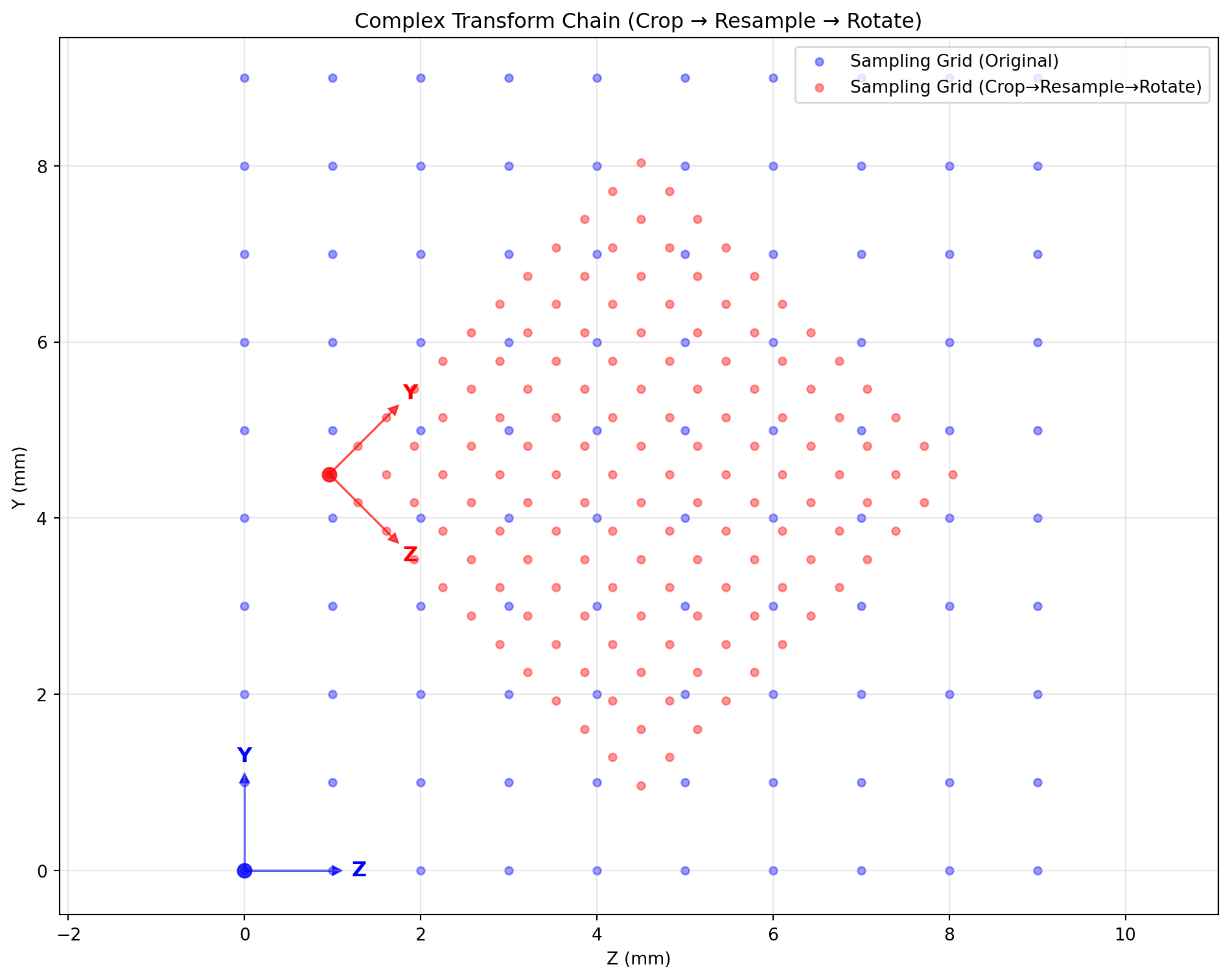

浮点边界框采样（float-point bbox sampling）

float_bbox_space = standard_space.apply_float_bbox(np.array([[0, 1], [2.5, 5.5], [2.5, 5.5]]), (12, 12, 12))

setup_plot()
visualize_sampling_grid(standard_space, color='blue', label_suffix=' (Original)')
visualize_sampling_grid(float_bbox_space, color='red', label_suffix=' (Float Bounding Box)')
finalize_plot('Float Bounding Box Sampling (6x6 ROI)')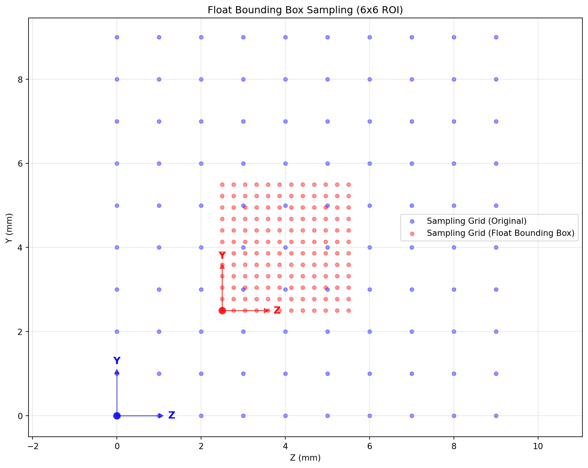

Space 抽象框架的核心优势

设计理念：Space 中心 vs Transform 中心

SpaceTransformer 采用“Space 中心”的设计理念，区别于 torchvision 等库的“Transform 中心”模式。该选择基于医学图像处理的本质：对象的坐标以世界坐标系为准。

Space 中心设计：每个数据对象（图像、点集、掩膜）都绑定唯一空间描述符。当两个对象需要对齐时，通过比较它们的 Space 属性自动生成精确变换关系。

Transform 中心的局限：变换本质相对，缺乏绝对基准，导致多对象空间关系难维护，容易产生累积误差。

技术实现：规划与执行分离

Space 类实现了空间变换的“规划阶段”与“执行阶段”完全解耦：

规划阶段：通过链式调用构建复杂变换序列，所有操作在抽象几何空间进行，无需触碰像素数据。

执行阶段：warp_image 分析完整变换链，自动选择最优插值路径，以单次采样完成全部变换。

实际收益

几何精度：变换顺序不影响结果。“旋转→缩放”与“缩放→旋转”在 Space 层面等价，避免传统方法受采样边界影响的信息丢失。

内存效率：消除多步骤变换中的中间缓存；传统每步都需要完整图像拷贝，而 Space 仅在最终执行时分配目标内存一次。

架构简洁：库中的 warp_xxx 接口处理所有类型变换，无需针对图像/点集/掩膜分别维护复杂逻辑。

接口易用：相比 SimpleITK 需手工配置采样参数，SpaceTransformer 提供语义化接口，同时保留高级用户的底层控制力。